There are a lot of different parts to an Excel spreadsheet and each part can be hidden in different ways. In this article, I’ll walk you through the different content that can be hidden in Excel and how to get view the hidden data at a later time.
How to Hide Tabs/WorkSheets
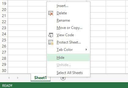
In order to hide a worksheet or tab in Excel, right-click on the tab and choose Hide. That was pretty straightforward.
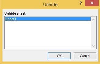
Once hidden, you can right-click on a visible sheet and select Unhide. All hidden sheets will be shown in a list and you can select the one you want to unhide.
How to Hide Cells
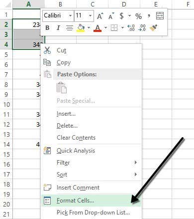
Excel does not have the ability to hide a cell in the traditional sense that they simply disappear until you unhide them, like in the example above with sheets. It can only blank out a cell so that it appears that nothing is in the cell, but it can’t truly “hide” a cell because if a cell is hidden, what would you replace that cell with? You can hide entire rows and columns in Excel, which I explain below, but you can only blank out individual cells. Right-click on a cell or multiple selected cells and then click on Format Cells.
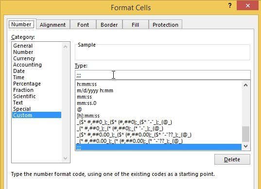
On the Number tab, choose Custom at the bottom and enter three semicolons (;;;) without the parentheses into the Type box.
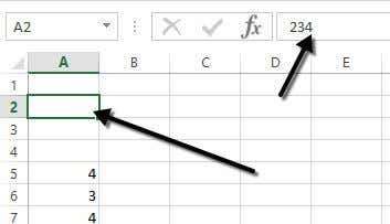
Click OK and now the data in those cells is hidden. You can click on the cell and you should see the cell remains blank, but the data in the cell shows up in the formula bar.
To unhide the cells, follow the same procedure above, but this time choose the original format of the cells rather than Custom. Note that if you type anything into those cells, it will automatically be hidden after you press Enter. Also, whatever original value was in the hidden cell will be replaced when typing into the hidden cell.
Hide Gridlines
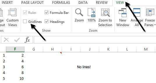
A common task in Excel is hiding gridlines to make the presentation of the data cleaner. When hiding gridlines, you can either hide all gridlines on the entire worksheet or you can hide gridlines for a certain portion of the worksheet. I will explain both options below. To hide all gridlines, you can click on the View tab and then uncheck the Gridlines box.
You can also click on the Page Layout tab and uncheck the View box under Gridlines.
How to Hide Rows and Columns
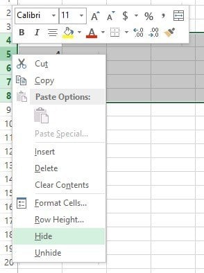
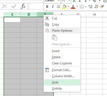
If you want to hide an entire row or column, right-click on the row or column header and then choose Hide. To hide a row or multiple rows, you need to right-click on the row number at the far left. To hide a column or multiple columns, you need to right-click on the column letter at the very top.
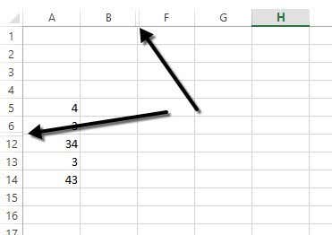
You can easily tell there are hidden rows and columns in Excel because the numbers or letters skip and there are two visible lines shown to indicate hidden columns or rows.
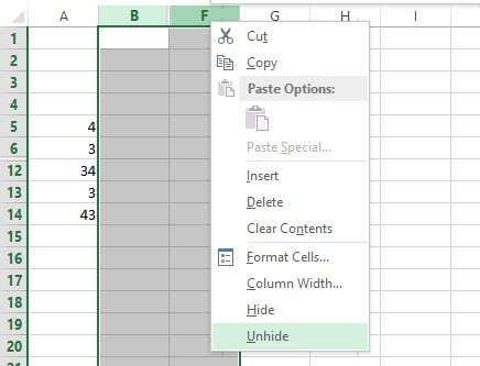
To unhide a row or column, you need to select the row/column before and the row/column after the hidden row/column. For example, if Column B is hidden, you would need to select column A and column C and then right-click and choose Unhide to unhide it.
How to Hide Formulas
Hiding formulas is slightly more complicated than hiding rows, columns, and tabs. If you want to hide a formula, you have to do TWO things: set the cells to Hidden and then protect the sheet. So, for example, I have a sheet with some proprietary formulas that I don’t want anyone to see!
First, I will select the cells in column F, right-click and choose Format Cells. Now click on the Protection tab and check the box that says Hidden.
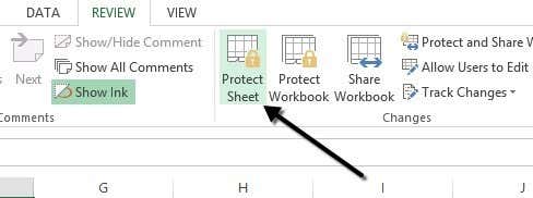
As you can see from the message, hiding formulas won’t go into effect until you actually protect the worksheet. You can do this by clicking on the Review tab and then clicking on Protect Sheet.
You can enter in a password if you want to prevent people from un-hiding the formulas. Now you’ll notice that if you try to view the formulas, by pressing CTRL + ~ or by clicking on Show Formulas on the Formulas tab, they will not be visible, however, the results of that formula will remain visible.
Hide Comments
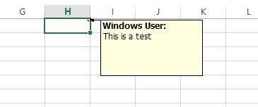
By default, when you add a comment to an Excel cell, it will show you a small red arrow in the upper right corner to indicate there is a comment there. When you hover over the cell or select it, the comment will appear in a pop up window automatically.
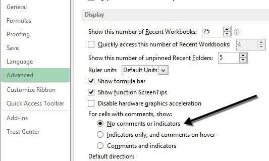
You can change this behavior so that the arrow and the comment are not shown when hovering or selecting the cell. The comment will still remain and can be viewed by simply going to the Review tab and clicking on Show All Comments. To hide the comments, click on File and then Options.
Click on Advanced and then scroll down to the Display section. There you will see an option called No comment or indicators under the For cells with comments, show: heading.
Hide Overflow Text
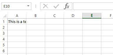
In Excel, if you type a lot of text into a cell, it will simply overflow over the adjacent cells. In the example below, the text only exists in cell A1, but it overflows to other cells so that you can see it all.
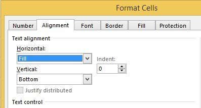
If I were to type something into cell B1, it would then cut off the overflow and show the contents of B1. If you want this behavior without having to type anything into the adjacent cell, you can right-click on the cell, choose Format Cells and then select Fill from the Horizontal Text alignment drop down box.
This will hide the overflow text for that cell even if nothing is in the adjacent cell. Note that this is kind of a hack, but it works most of the time.
You could also choose Format Cells and then check the Wrap Text box under Text control on the Alignment tab, but that will increase the height of the row. To get around that, you could simply right-click on the row number and then click on Row Height to adjust the height back to its original value. Either of these two methods will work for hiding overflow text.
Hide Workbook
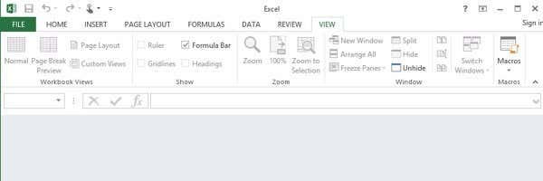
I’m not sure why you would want or need to do this, but you can also click on the View tab and click on the Hide button under Split. This will hide the entire workbook in Excel! There is absolutely nothing you can do other than clicking on the Unhide button to bring back the workbook.
So now you’ve learnt how to hide workbooks, sheets, rows, columns, gridlines, comments, cells, and formulas in Excel! If you have any questions, post a comment. Enjoy!
